The CPA Revolution: Intro Series PwrPvt

Showing posts with label Intro Series PwrPvt. Show all posts

What's killing My Excel?

Across the globe, Excel crashing is an accountant or analyst's bane. I've been there and know how exhausting it can be. Fortunately (knock on wood), I've found some tips which have virtually eliminated crashing for me.

Get 64-bit Excel

Disable add-ins

Prioritize Excel

Check your resource monitor

Get 64-bit Excel

The #1 way to fix Excel crashing issues is to install the 64-bit version of Excel on Office 365.

By default, IT departments across the globe install the 32-bit version of Excel on Office 365. While that works for most, Excel's 32-bit version is not sufficient for running the more complex Excel workbooks used by finance and accounting teams. See this Microsoft Office article about why multiple Pivot Tables, slicers and VLOOKUPs can constrain your Excel resources.

Finance and Accounting users are frequently the largest Excel consumers, but your IT support team may not realize it when deploying PCs to users. If your Finance and Accounting teams aren't using 64-bit Excel today, there may be some support team resistance to making the change and deploying 64-bit. Historically, Microsoft Office recommended 32-bit installs by default; however, it did not apply to power users like Finance and Accounting teams. Here's a link to another Microsoft Office article which might help persuade.

Incapability with existing add-ins, such as Hyperion Essbase, is the primary issue which may need to be addressed.

First, I recommend seeing if there is a 64-bit version of your add-in.
If not, consider installing anyway and testing the impact.
If impacted, explore with your IT team other solutions, such as a 32-bit Excel version with the add-in installed inside a Citrix environment and the 64-bit Excel version on your desktop.

If you are experiencing install setbacks, don't give up; I assure you the 64-bit version is worth it. While you wait for IT to validate add-ins, try one of the other solutions below.

Disable Add-Ins

Excel Add-ins sometimes behave badly, especially when the version of Excel the add-in was built on and the current user version of Excel deviate. This seems to be especially true in the Office 365 environment where updates can occur monthly.

Initially, try disabling all add-ins and turning them on only when needed. To effectuate, in Excel go to File, Options, Add-ins, Manage, Excel Add-ins, Go. Uncheck all the add-ins. Next, repeat these steps, but select Manage, COM Add-ins, Go.

💥BEST PRACTICE TIP
Speed up the add-in disabling process by adding a short-cut to your Excel Quick Access Toolbar. In Excel, go to File, Options, Quick Access Toolbar, Choose commands from: All Commands, Add-ins (the first one, which has no icon & a drop down menu). 💥

When Excel crashes, keep track of which add-ins, if any, were enabled. Once an add-in has been identified as a culprit, work with your IT team to address. In the meantime, whenever you need to enable the suspect add-in, save backup copies often.

If Excel crashes at the same frequency when the add-ins are disabled, then add-ins is likely not your primary culprit; read further and see if one of the other solutions helps.

Prioritize Excel

All running applications share processor time. Tell your computer to give Excel more love by changing the priority level.

Use Ctrl+Alt+Del to open Task Manager. On the Details tab, right click on Excel.exe process. Choose Set Priority. Then, select either High or Above Normal.

The priority auto-resets to Normal whenever Excel is restarted making this a temporary solution at best.

While it may be tempting to choose Real Time, rumor has it that this will make your other applications jealous, your CPU's head spin, and your PC crash. 💔

Check your resource monitor

Return to Task Master. On the bottom of the Performance tab, select "Open Resource Monitor". This tool provides utilization visuals for the processes running on your machine. Choose the Overview tab and keep the 4 charts open and visible while you work. When the Resource Monitor charts are at their maximums for an extended period of time, drill down on the applicable Resource Monitor tab to try and isolate what is dragging you down. With data in hand, partner with IT support to achieve improved performance.

In this lesson, you learned how to eliminate Excel crashes by:

Installing 64-bit Excel,

Disabling add-ins,

Prioritizing Excel, and

Checking your resource monitor.

Prior post: Measures Inside Measures
Next post: Distinguishing datasets in Power Pivot

💬Always love hearing how others have tackled Excel performance issues. Drop a comment below to share.

Measures inside Measures

This is the final post of the Intro to Power Pivot series. Jump to the 1st post of the series here.

It's time to wrap up the Intro to Power Pivot series. This post will work through writing the final three Measures (Var to Budget, Prior Year, and Var to PY).

Budget variance

Let's calculate the variance between Actual and Budget by month.

Start with the workbook created from the last exercise, Measures In-depth, or download this file.
With your cursor in the Pivot Table, go to the Power Pivot menu, and select Measures, New Measure.

In the Measure dialog box, select the Table, Actual_Data.
Change the Measure name to Var to Budget.
In the formula box, type =[Actual] - [Budget].

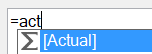
Start typing Actual, and you will get a drop down box to select from.
Measures have a 𝚺 sign next to them and are noted in brackets.
Press Tab to select.

Check formula. Result should be no errors.
Format by changing the Category to Number, with 0 decimal places.
Ok.

Prior Year Measure using CALCULATE

Let's create a Prior Year Measure to show the 2012 Actual values. The formula for creating that Measure is as follows:

= CALCULATE ( [Actual] , Date_LU[Year] = 2012 )

The CALCULATE function can filter a Measure. The CALCULATE function requires first, the Measure, and then the filter. The Measure is [Actual]. The filter is the 2012 year, which is pulling from the Year column of the Lookup Table, Date_LU. Columns and Measures are in brackets.

Notice how the Prior Year column is showing the 2012 Actual numbers for both 2012 and 2013. Using CALCULATE you've told Excel to always show the 2012 actual value regardless of the year presented in the Pivot Table. This is referred to as filter context and occurs because CALCULATE filters take precedent over Pivot Table filters.

💥BEST PRACTICE TIP
CALCULATE is a very powerful function. Always test that the results are as expected. If others in your organization aren't using Power Pivot yet, consider adding a comment to alert the user to the CALCULATE function. 💥

Pivot

Let's do some quick clean-up before moving on to our final Measure.

In the PivotTable Fields List, move the Year field from Columns to Filters. Filter to show only 2013.
In the Values area, move Prior Year to the top, so it is the first column in the Pivot.

Variance to Prior Year Measure

For our final Measure, let's write the variance to the prior year.

Below is a screenshot of the final result.

By the time you wrote your 5th and final Measure for this Intro to Power Pivot series, hopefully, you were starting to get the flow for Measures. Keep practicing, replacing your normal SUM of Values with Measures and trying out a few CALCULATE exercises. Pretty soon Power Pivot will be second nature.

In this lesson, you learned how to:

Write Measures which reference other Measures;
Write Measures to take the difference between columns in a Pivot Table; and,
Use the CALCULATE formula to create filtered values.

SOLUTION

Prior post: Measures In-Depth
Next post: What's killing my Excel?

Measures in-depth

This is the 7th post of the Intro to Power Pivot series. Jump to the 1st post of the series here.

Below is the Pivot Table from the last exercise. Let's create the Measure, Actual, and polish up the Table. Then, let's talk more in-depth about Measures.

Writing the Actual Measure

Start with the workbook created from the last exercise, Measures, or download this file.

With your cursor in the Pivot Table, go to the Power Pivot menu, and select Measures, New Measure.

In the Measure dialog box, select the Table, Actual_Data.
Change the Measure name to Actual.
In the formula box, type =SUM(Actual_Data[Sales]).
Check formula. Result should be no errors.
Format by changing the Category to Number, with 0 decimal places.
Ok.

Your Pivot Table now contains the new Measure "Actual". You can compare to the Sum of Sales values you are accustomed to seeing and confirm the Measure resulted in the same output (just formatted).

In the Values area of the PivotTable Fields List, remove both the Sum of Sales metrics. Below is a snapshot of the Pivot Table, which now contains the two Measures, Budget and Actual.

Measures In-depth

With the introduction of Measures, you've unleashed a tremendous amount of calculating power, which hasn't yet been explained. Let's revisit each element of the Measures dialog box to start digging deeper.

Table Name

The Table Name selected determines where a Measure is located on the Fields section of the PivotTable Fields List. Note the Actual and Budget Measures in the image below.

Some people recommend placing Measures on the queries where the related data sits, which was the structure selected for this exercise. Selecting the queries to assign a Measure to is a matter of personal preference. The Measure will return the same result regardless of the query assigned.

Measure Name

The Measure Name will be the default displayed name on the Pivot Table, as Budget and Actual are in our exercise. Like a normal Pivot Table, the displayed name can be changed in Value Field Settings. In the example below, the Measure Name would be "Actual" and the displayed name on the Pivot would be "Actual Sales".

Name your Measures something intuitive to make it clear what the Measure is calculating. As your Data Models start to have multiple Measures, such as Actual Sales and Actual Orders, it will be helpful to easily distinguish between the two. In our Data Model, Actual Sales and Budgeted Sales would have been more robust Measure names than Actual and Budget.

💥BEST PRACTICE TIP
Create robust Measure names. Think about possible future uses for your Data Model. Changing a Measure name later can cause headaches. A renamed Measure is removed from any existing Pivot Tables and requires modifying any dependent Measures. 💥

Formula

The formula area is the meat of the Measure and where the DAX language comes in to play. Measures are calculations which display in the Values area of a Pivot Table. As a calculation, Measures always start with an equal sign.

=SUM(Actual_Data[Sales])

The next element is the function. There are more than 200 DAX functions, many which resemble functions in native Excel, but give more Power to your analytics.

In our exercise, we used the function SUM. SUM adds up the amounts in a specified column. All functions are followed by an open and closed parenthesis: =SUM().

For the SUM function, we specified the column as Actual_Data[Sales] surrounded by open and closed parenthesis. Since Data Models can contain multiple tables (queries) which can have the same column names (such as Sales), when specifying a column, include the table name and the column name. Our table name was Actual_Data, and the column we are summing from that table is Sales. Columns are referenced in brackets.

At this point, we've comparatively done a lot of work to mimic the "Sum of Sales" value normally included in a Pivot Table. This is a simple example, designed to mimic something you are likely very familiar with to lay the foundation for more complex Measures and analysis.

As an additional foundational exercise, I recommend reviewing the official documentation for a formula: Microsoft link. As you venture on your own, understanding how non-accountants reference the elements of a function enhances collaboration.

Check formula

After writing the formula, Always press "Check formula". The green checkmark and "No errors in formula" message confirm the formula is written correctly.

A very common error message is the following, unhelpful message.

When the above message is received, check to make sure there is a closed parenthesis at the end of the formula.

Using Tab and the drop down menus can assist with dropping in the function and column names correctly. Unlike Power Query, DAX is not case sensitive.

Format

When viewing the Measures "Budget" and "Actual" in your Pivot Table, you may have noticed they were formatted with a comma and no decimals.

This was based on the format settings listed in the Measure dialog box. Each time a Measure is used, the format is set and ready to go.

In this lesson, you:

Practiced writing Measures;
Compared Measures to the traditional approach of adding Values to a Pivot;
Explored each component of the Measure dialog box;
Learned how to write robust Measure names; and,
Resolved common Measure errors.

There's a lot more to talk about regarding Measures. Subscribe below to be alerted when the next post is ready.

SOLUTION

Prior post: Measures
Next post: Measures inside Measures

💬 Challenge exercise:
Load the Actual_Data query in to PowerBI, and write the Actual Measure, =SUM(Actual_Data[Sales]).

Measures

This is the 1st post on Measures and the 6th post of the Intro to Power Pivot series. Jump to the 1st post of Power Pivot series here.

Measures allow the creation of custom formulas to harness big data using Power Pivot. Measures use a formula language called Data Analysis Expressions (DAX). Many DAX formulas are similar to native Excel, such as SUM, but they extract the value from a table, column, or subset of your data, instead of referencing cell ranges, and they can be used across your Data Model.

Writing a Measure

Start with the workbook created from the last exercise, 2 Data Tables on 1 Pivot Table, or download this file.

The Pivot Table in the file currently has two values named Sum of Sales, which is not helpful. Using Measures, let's create more meaningful descriptors, such as Budget and Actual.

With your cursor in the Pivot Table, go to the Power Pivot menu, and select Measures, New Measure.

In the Measure dialog box, select Budget_Data as the Table name.
Change the Measure name to Budget.
In the formula box, type =SUM(Budget_Data[Sales]).
Change the Category to Number, with 0 decimal places.

The Pivot Table now contains the new Measure "Budget".

Learning Curves

Not everyone got that result on the first try. Let's talk about a few things that could have thrown you a curve, and how to fix them.

Measure not on Pivot Table

If the Budget Measure is not on the Pivot Table at all, it's because the cursor was not in the Pivot Table when New Measure was selected from the Power Pivot ribbon. Go to the Pivot Table Fields List, and locate the fx Budget checkbox. Check the box, and the new Measure is added to the Pivot.

Measure in different section of Fields List

If the new Measure is not listed under Budget_Data, in the Fields List search box, type Budget. Check the box to add the Measure to the Pivot. This occurs when the Table Name used in the Measure was something other than Budget_Data.

Measure Name or Formatting is incorrect

If the Measure is on the Pivot Table, but it's not named Budget or formatted with a comma and no decimals, then the Measure needs to be modified by reopening the Measure dialog box. On the Power Pivot menu, select Measures, Manage Measures and modify to match the image above.

In this lesson, you learned:

What a Measure is;
How to write a Measure; and,
Troubleshooting for common Measure problems.

SOLUTION

Prior post: 2 Data Tables on 1 Pivot Table
Next post: Measures In-depth

2 Data Tables on 1 Pivot Table

This is the 5th post of the Intro to Power Pivot series. Jump to the 1st post of the series here.

This lesson walks through the steps to load the 2^nd Data Table (Actual), build a relationship to the Lookup Table, and add actual sales to the budgeted sales Pivot Table.

Load the Actual Data Table

Start with the workbook created from the last exercise, Building Relationships, or download this file.

Load the Actual data to the exercise workbook by performing the following steps:

Download the Actual file by selecting the Download icon below.

↑

In the exercise workbook, go to the Data tab, Get Data, From File, From Workbook.
Browse to select the downloaded Actual file and Import.
On the Navigator, select the Table, then Transform Data (or Edit).
Rename the Query, Actual_Data.

Establish a common field

The Actual file lists actual sales by day in the format MM/DD/YYYY, The Date Lookup Table is rolled up to the monthly level. Therefore, we need to create a column in the Actual query that we can build a relationship with.

Choose the Date of Sale column, and then on the Add Column tab, select Date, Month, Start of Month.

The query is now loaded and transformed. Go to the Close & Load drop down menu, Close & Load To, Only Create Connection, Add this data to the Data Model and select Ok.

Build a relationship

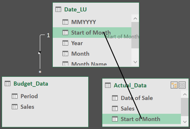
In the Power Pivot menu, select Manage to open Power Pivot. On the Home tab, select Diagram View.

Rearrange the Actual_Data query so the Data Table looks up to the Lookup Table.

On the Actual_Data box, select the Start of Month and drag up to the Start of Month on the Date_LU.

The connector should indicate a 1 next to the Date_LU Table, since this Table holds unique values.

Close Power Pivot.

💥BEST PRACTICE TIP
Always connect the Data Table to the Lookup Table. Do not connect Data Tables to each other.💥

Pivot Budget and Actual on 1 Pivot Table

In the Pivot Table Field List, there are now 3 queries to choose from including Actual_Data.

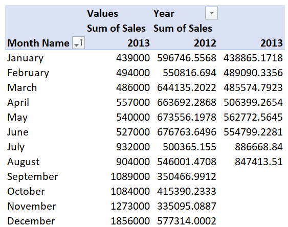
Add Sales from the Actual_Data query to the Pivot Table Value section. Remove from Rows the Period field from the Budget_Data query. Also, from the Date_LU remove from Rows the Start of Month and Month, and add to Columns the Year.

With the cursor in the Month Name column of the Pivot Table, right click and Sort by Ascending.

It's not polished yet, but the goal has been achieved. The Pivot Table reflects 2 Data Tables and two different sales figures: budget and actual.

In this lesson, you learned how to:

Handle relationships when there are two Data Tables; and
Pivot 3 data sets on 1 Pivot Table.

SOLUTION

Prior post: Building relationships
Next post: Measures

Building relationships

This is the 4th post of the Intro to Power Pivot series. Jump to the 1st post of the series here.

In this lesson, you will load the 1st Data Table, build the 1st relationship, and create a Pivot Table using both the Lookup and the 1st Data Table.

Load the Budget Data

Open the workbook you created in the last exercise, Power Pivot Date Table, or download the file here.

Load the budget data to the workbook by performing the following steps:

Download the budget file below.
In the exercise workbook, go to the Data tab, Get Data, From File, From Workbook.
Browse to select the downloaded budget file and Import.
On the Navigator, select the Budget Table, then Transform Data (or Edit).
Rename the Query, Budget_Data.
Close & Load drop down menu, Close & Load To, Only Create Connection, Add this data to the Data Model. Ok.

↑

First Look at Power Pivot

We've loaded two files to our Data Model. It's time to move from Power Query to Power Pivot.

In the Power Pivot menu, select Manage. This opens Power Pivot. Alternatively, you can also access Power Pivot by selecting the smaller version of the Manage icon, in the Data Tools section of the Data menu.

When Power Pivot opens, the initial view is called the Data view. In this view, you will see on separate tabs each of the queries loaded to the Data Model.

Think of this as a read only view, as the original queries can only be modified at the source or in Power Query.

On the Home tab, select Diagram View.

The diagram view shows the column names of each query and is a place to visualize how your queries relate to each other.

First, let's rearrange the queries so the Data Table looks up to the Lookup Table. Rearrange by dragging the Budget_Data box under the Date_LU box. I call this the Golden rule of Power Pivot; it's more commonly referred to as the Collie method, for the creator, Rob Collie of PowerPivotPro.com. Visualize how in the image below the Data Table looks up to the Lookup Table.

💥BEST PRACTICE TIP
Layout your Data Model, so the Data Tables look up to the Lookup Tables.💥

Build a relationship

Next, we are going to connect the queries together based on a common field.

For this Data Model, the Date_LU query column MMYYY equates to the Period column in the Budget_Data query.

To connect the two columns, select Period, and while holding down the left mouse button, drag your cursor to MMYYYY. A line illustrates the connection being built between Period and MMYYYY.

After the two queries are connected, a connector is displayed.

The connector tells us several important things:

Placing your cursor on the connector highlights which columns the connections were made on.
The downward direction of the arrow on the connector tells us the Lookup Table is flowing the value down to the Data Table.
The "1" indicates that the values in the MMYYYY column are unique (no two values are the same). The * indicates that the values in the Period column can be any value. This is referred to as a "One-to-Many Relationship" and is a key concept in building Data Models with Power Pivot.

Building a relationship vs. using VLOOKUP

In a traditional VLOOKUP, you would lookup the data from the Lookup Table and add it to the Data Table. Using Power Pivot, you tell Excel where to look for the value but don't copy the value to the Data Table. This saves enormous resources and dramatically decreases file size and improves calculation speeds.

A Pivot Table with 2 tables

Now that the relationship is built, close Power Pivot.

Insert a Pivot Table, selecting "Use this workbook's Data Model".

Great news! Power Pivot uses the same Pivot Table that you already know and love. Everything looks the same as it did before, with one exception. In the Pivot Table Field List, there are now multiple data sets available to choose from. I get shivers thinking about how this simple change dramatically transformed my work and improved my efficiency.

From the Budget_Data query, place Period in Rows and Sales in the Values area of the Pivot.

Previously, this Pivot Table yields all the data we would have been able to extract from the budget file. If we wanted to add, Year, Month, and Month Name we would need to add 3 new columns to the budget file (and repeat each time we received a new file from the budget team).

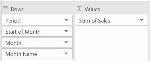
Let's look at how the world has changed. In the Pivot Table Fields List, add Start of Month, Month and Month Name to rows.

If you do nothing else in Power Pivot, when your Lookup Table has unique values, load your files and build the relationships to remove VLOOKUPs. You will find immediate improvement in the performance of your files.

The Power Pivot Data Model compresses data 7 to 10 times smaller than the same data in native Excel. Native Excel uses the in-memory analytics engine to store data in memory (hence why large files with complex formulas or multiple Pivots receive resource error messages).

In this lesson, you learned how to:

Navigate in Power Pivot;
Build relationships using Power Pivot;
Interpret the Connector in Power Pivot;
Create 1 Pivot Table using 2 data sets; and,
The value of performing calculations, such as VLOOKUP, in Power Pivot instead of native Excel.

SOLUTION

Prior post: Power Pivot Date Table
Next post: 2 Data Tables on 1 Pivot Table

💬 Questions or challenges can always be addressed in the comment section below.