Showing posts with label Measures. Show all posts

Measures: Right & Wrong

Explore prior lessons on Measures here.

Measures are very powerful custom functions used inside Pivot Tables.  However, when I started using them, I found myself getting easily twisted up between when to use SUM vs SUMX.

I built a cheat sheet to help me remember.  Hope it helps you too.


The Cheat Sheet

Table1 below has Qty & Price. To calculate Sales, you could add a column to multiple Qty * Price as shown.  However, calculating a value for each row uses a lot of memory, especially when you have lots of data.
Measures are a much more efficient way to calculate values for large data sets. There are several ways to write Measures to calculate sales, but only one way which avoids adding the Sales column to the Table above and results in the correct Grand Total of 20.

Note first, in all cases the sales for Item A have been calculated correctly, as well as Item B.  The difference is the Grand Total. Adding 11 to 9 is 20, so with this small dataset this is an easy approach to check if a Measure is returning the correct result.
  
Sum of Sales
Sum of Sales was calculated the traditional way, by pulling the Sales column in to the Values section of the Pivot Table.  It achieves the correct result. However, it can't be inserted inside another function such as Item Sales as a % of Total Sales.  It also requires having a Sales column in the Table which isn't efficient.

Sales SUM
The next approach does not need a Sales column in the Table.  This is a Measure which multiplies Price times Qty.  This yields the correct result for the Sales of Items A and B, but the Grand total takes the combined price of Items A & B (11+3=14) times the combined Qty (1+3=4), which equals 14*4=56.  This is incorrect as the sum of the sales for A (11) & B (9) is 20.

Sales Sum of Sum

When writing a Measure for the first time, I like starting with something I know will work and then building out from there. The Sales Sum of Sum utilizes the Sales column that was added to Table1. Taking the Sum of the Sales column yields the correct Grand Total.  However, having an extra column isn't ideal.  

Sales SUMX


SUMX is an iterator: it goes through each row and sums it. First the Sum of the Sales column was calculated, which was 20, then SUMX went through each row of the query and summed the sales.  Effectively, this doubled each Item's sales. Using the Sales column in Table1, SUMX summed the total sales in row A & B, essentially doubling total sales.  Wrong answer but an iterator has potential.

SUMX Sales


Now that's the right answer! But, it's using the Sales column again.  However, it does tell us that SUMX could be used to get to the correct subtotal.  

SUMX PQ


Finally, the sweet spot. SUMX PQ has the correct Grandtotal and does not require a Sales column added to the Table.  This is the correct way to write a SUMX Measure.

Wrap-up

This cheat sheet shows all the wrong ways to write a Measure. When I tried to write DAX on the fly in the beginning, I've made every one of these errors. Happy DAX-ing!  

In this lesson, you learned how to:
  • Write SUMX Measures the wrong way, and
  • Write SUMX Measures the right way. 


Prior post: M-language

Calculated columns vs Measures


Just joining the blog? Explore prior lessons here.

When playing with the Power tools, there is often more than one way to tackle a task. Read further to explore the pros and cons of calculated columns and Measures. 

For this exercise, we'll use the dataset below to find Total Sales for each product using calculated columns and then a Measure. 
       
                                    ⇧


Calculated Column

A calculated column expands a dataset by adding an additional column. It's similar to native Excel where you would write a formula in a new column.

New users will feel more comfortable using calculated columns instead of Measures. However, there are some downsides to this approach which we'll explore further down. For now though, let's practice our Power Query skills by adding a calculated column.

Select the Download icon above the arrow ⇧ on the dataset above.  With your cursor in the Table, load to Power Query by going to the Data tab and selecting From Table/Range.  

Inside the Power Query Editor, on the Add Column tab, select Custom Column. 

Create a "Total sales" column like the example below.

After selecting OK, the new Calculated Column has been added to our query.


Change the type of "Total sales" to Decimal Number and then Close & Load To, Table, New worksheet, Add this data to the Data Model, Load.

Advantages of using Power Query instead of native Excel to build the Calculated Column include:
  • Removes the potential for a formula to get altered accidentally;
  • Shrinks the file size, since Power Query uses xVelocity to compress data; and,
  • Allows processing of massive amounts of data since Power Query is limited only by the capacity of your machine, not Excel's ~1 million rows limit: 20 million rows, no problem.
However, it could be even better. Let's try it in Power Pivot.


Build a Power Pivot Pivot Table

Before we write a Measure, let's add a Pivot Table to our workbook, so we can see the results. 

Choose to "Use this workbook's Data Model".  This creates a Pivot Table using the data loaded in to Power Query.

In the PivotTable Fields, there may be 3 Sales_data sets to choose from when selecting fields for the Pivot.  

Hovering over the name yields more information to distinguish between the data sources.
  • The first is the original Data Table which was loaded to Power Query.
  • The second is the query that was created in Power Query.
  • The third is the output of the query.
On the PivotTable Field List, select from the query "Sales_data 1" and pull Product in to the Rows area and "Total sales" in to the Values area.


Measure

Now, let's calculate Total Sales again, but this time using a Measure instead of a calculated column. The results will be the same, but Measures have additional advantages over native Excel and calculated columns.

The Measure will need to multiply Qty and Unit Price for each row of the data and then sum those products to get a grand total.  To achieve this result, we will use a SUMX formula, which is an iterator formula, which iterates through each row of the Table and then sums the total.

The SUMX format is 
    = SUMX(Source Query, function to perform on each row before summing)
In our case, this roughly translates to
    =SUMX(Sales_data 1, Qty*Unit Price)

Let's write the Measure. 

On the Power Pivot menu, select Measures, New Measure.

  •  Name the Measure, "Total sales Measure". 
  • Start the formula with an equal sign.
  • SUMX first needs a table to reference, so type an open parenthesis, then 'Sales_data 1' followed by a comma.
  • Then, start the expression by typing Qty.  Select 'Sales_data 1'[Qty], which is the quantity column from the query. 
  • Add a multiplication sign.
  • Type "price" and then select 'Sales_data 1'[Unit Price].
  • Close parenthesis.
Check the formula and assign the value a category.  Here's the solution.
=SUMX('Sales_data 1','Sales_data 1'[Qty]*'Sales_data 1'[Unit Price])
Return to your Pivot Table, and add in the new Measure.

Advantages of using Power Pivot Measures instead of native Excel or Power Query to build the Total Sales calculation include:
  • All the advantages listed above for calculated columns versus native Excel plus the following.
  • Measures use less memory than calculated columns.
  • The Power Pivot Data Model compresses data 7 to 10 times smaller than the same data in native Excel.  
    • Native Excel uses the in-memory analytics engine to store data in memory (hence why large files with complex formulas or multiple Pivots receive resource error messages).
  • Measures can be reused in multiple Pivot Tables in the same workbook.
  • Measures can be referred to in other Measures. For example, if we had to add sales tax of 10%, a Measure could be written to take =Total Sales Measure * 10%.
MeasureNow, let's calculate Total Sales again, but this time using a Measure instead of a calculated column. The results will be the same, but Measures have additional advantages over native Excel and calculated columns.

The Measure will need to multiply Qty and Unit Price for each row of the data and then sum those products to get a grand total.  To achieve this result, we will use a SUMX formula, which is an iterator formula, which iterates through each row of the Table and then sums the total.

The SUMX format is 
    = SUMX(Source Query, function to perform on each row before summing)
In our case, this roughly translates to
    =SUMX(Sales_data 1, Qty*Unit Price)

Let's write the Measure. 

On the Power Pivot menu, select Measures, New Measure.

  • Name the Measure, "Total sales Measure".
  • Start the formula with an equal sign.
  • SUMX first needs a table to reference, so type an open parenthesis, then 'Sales_data 1' followed by a comma.
  • Then, start the expression by typing Qty. Select 'Sales_data 1'[Qty], which is the quantity column from the query.
  • Add a multiplication sign.
  • Type "price" and then select 'Sales_data 1'[Unit Price].
  • Close parenthesis.
Check the formula and assign the value a category.  Here's the solution.
=SUMX('Sales_data 1','Sales_data 1'[Qty]*'Sales_data 1'[Unit Price])
Return to your Pivot Table, and add in the new Measure.

Advantages of using Power Pivot Measures instead of native Excel or Power Query to build the Total Sales calculation include:
  • All the advantages listed above for calculated columns versus native Excel plus the following.
  • Measures use less memory than calculated columns.
  • The Power Pivot Data Model compresses data 7 to 10 times smaller than the same data in native Excel.  
    • Native Excel uses the in-memory analytics engine to store data in memory (hence why large files with complex formulas or multiple Pivots receive resource error messages).
  • Measures can be reused in multiple Pivot Tables in the same workbook.
  • Measures can be referred to in other Measures. For example, if we had to add sales tax of 10%, a Measure could be written to take =Total Sales Measure * 10%.

In this lesson, you learned:
  • Calculated columns and Measures can return the same results;
  • The difference between creating a calculated column and a Measure;
  • The advantages of creating a Power Query calculated column instead of using native Excel; and,
  • The advantages of creating Measures instead of using native Excel or Power Query.

SOLUTION 


Prior post: The Power of the Unpivot
Next post: M-language

Measures inside Measures

This is the final post of the Intro to Power Pivot series.  Jump to the 1st post of the series here.


It's time to wrap up the Intro to Power Pivot series.  This post will work through writing the final three Measures (Var to Budget, Prior Year, and Var to PY).


Budget variance

Let's calculate the variance between Actual and Budget by month.

Start with the workbook created from the last exercise, Measures In-depth, or download this file.
With your cursor in the Pivot Table, go to the Power Pivot menu, and select Measures, New Measure.


In the Measure dialog box, select the Table, Actual_Data.
Change the Measure name to Var to Budget.
In the formula box, type =[Actual] - [Budget].


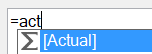
Start typing Actual, and you will get a drop down box to select from.
Measures have a 𝚺 sign next to them and are noted in brackets.
Press Tab to select.

Check formula.  Result should be no errors.
Format by changing the Category to Number, with 0 decimal places.
Ok.


Prior Year Measure using CALCULATE

Let's create a Prior Year Measure to show the 2012 Actual values.  The formula for creating that Measure is as follows:

= CALCULATE ( [Actual] , Date_LU[Year] = 2012 )

The CALCULATE function can filter a Measure.  The CALCULATE function requires first, the Measure, and then the filter.  The Measure is [Actual].  The filter is the 2012 year, which is pulling from the Year column of the Lookup Table, Date_LU.  Columns and Measures are in brackets.


Notice how the Prior Year column is showing the 2012 Actual numbers for both 2012 and 2013.  Using CALCULATE you've told Excel to always show the 2012 actual value regardless of the year presented in the Pivot Table. This is referred to as filter context and occurs because CALCULATE filters take precedent over Pivot Table filters


πŸ’₯BEST PRACTICE TIP
CALCULATE is a very powerful function.  Always test that the results are as expected.  If others in your organization aren't using Power Pivot yet, consider adding a comment to alert the user to the CALCULATE function. πŸ’₯

Pivot

Let's do some quick clean-up before moving on to our final Measure.

In the PivotTable Fields List, move the Year field from Columns to Filters.  Filter to show only 2013.
In the Values area, move Prior Year to the top, so it is the first column in the Pivot.

Variance to Prior Year Measure 

For our final Measure, let's write the variance to the prior year.


Below is a screenshot of the final result.  


By the time you wrote your 5th and final Measure for this Intro to Power Pivot series, hopefully, you were starting to get the flow for Measures. Keep practicing, replacing your normal SUM of Values with Measures and trying out a few CALCULATE exercises. Pretty soon Power Pivot will be second nature.

In this lesson, you learned how to:
  • Write Measures which reference other Measures;
  • Write Measures to take the difference between columns in a Pivot Table; and,
  • Use the CALCULATE formula to create filtered values.

Measures in-depth


This is the 7th post of the Intro to Power Pivot series.  Jump to the 1st post of the series here.


Below is the Pivot Table from the last exercise.  Let's create the Measure, Actual, and polish up the Table.  Then, let's talk more in-depth about Measures.

Writing the Actual Measure

Start with the workbook created from the last exercise, Measures, or download this file.

With your cursor in the Pivot Table, go to the Power Pivot menu, and select Measures, New Measure.


In the Measure dialog box, select the Table, Actual_Data.
Change the Measure name to Actual.
In the formula box, type =SUM(Actual_Data[Sales]).
Check formula.  Result should be no errors.
Format by changing the Category to Number, with 0 decimal places.
Ok.

Your Pivot Table now contains the new Measure "Actual".  You can compare to the Sum of Sales values you are accustomed to seeing and confirm the Measure resulted in the same output (just formatted).  
In the Values area of the PivotTable Fields List, remove both the Sum of Sales metrics.  Below is a snapshot of the Pivot Table, which now contains the two Measures, Budget and Actual.

Measures In-depth

With the introduction of Measures, you've unleashed a tremendous amount of calculating power, which hasn't yet been explained.  Let's revisit each element of the Measures dialog box to start digging deeper.


Table Name

The Table Name selected determines where a Measure is located on the Fields section of the PivotTable Fields List.  Note the Actual and Budget Measures in the image below.

Some people recommend placing Measures on the queries where the related data sits, which was the structure selected for this exercise.  Selecting the queries to assign a Measure to is a matter of personal preference.  The Measure will return the same result regardless of the query assigned.    

Measure Name

The Measure Name will be the default displayed name on the Pivot Table, as Budget and Actual are in our exercise.  Like a normal Pivot Table, the displayed name can be changed in Value Field Settings.  In the example below, the Measure Name would be "Actual" and the displayed name on the Pivot would be "Actual Sales".

Name your Measures something intuitive to make it clear what the Measure is calculating.  As your Data Models start to have multiple Measures, such as Actual Sales and Actual Orders, it will be helpful to easily distinguish between the two.  In our Data Model, Actual Sales and Budgeted Sales would have been more robust Measure names than Actual and Budget.

πŸ’₯BEST PRACTICE TIP
Create robust Measure namesThink about possible future uses for your Data Model.  Changing a Measure name later can cause headaches.  A renamed Measure is removed from any existing Pivot Tables and requires modifying any dependent Measures.  πŸ’₯


Formula

The formula area is the meat of the Measure and where the DAX language comes in to play.  Measures are calculations which display in the Values area of a Pivot Table.  As a calculation, Measures always start with an equal sign.  

=SUM(Actual_Data[Sales])

The next element is the function.  There are more than 200 DAX functions, many which resemble functions in native Excel, but give more Power to your analytics.

In our exercise, we used the function SUM.  SUM adds up the amounts in a specified column.  All functions are followed by an open and closed parenthesis: =SUM().

For the SUM function, we specified the column as Actual_Data[Sales] surrounded by open and closed parenthesis.  Since Data Models can contain multiple tables (queries) which can have the same column names (such as Sales), when specifying a column, include the table name and the column name.  Our table name was Actual_Data, and the column we are summing from that table is Sales.  Columns are referenced in brackets.

At this point, we've comparatively done a lot of work to mimic the "Sum of Sales" value normally included in a Pivot Table.  This is a simple example, designed to mimic something you are likely very familiar with to lay the foundation for more complex Measures and analysis.     

As an additional foundational exercise, I recommend reviewing the official documentation for a formula: Microsoft link.  As you venture on your own, understanding how non-accountants reference the elements of a function enhances collaboration.  

Check formula

After writing the formula, Always press "Check formula".  The green checkmark and "No errors in formula" message confirm the formula is written correctly.

A very common error message is the following, unhelpful message.
When the above message is received, check to make sure there is a closed parenthesis at the end of the formula.

Using Tab and the drop down menus can assist with dropping in the function and column names correctly.  Unlike Power Query, DAX is not case sensitive.  

Format

When viewing the Measures "Budget" and "Actual" in your Pivot Table, you may have noticed they were formatted with a comma and no decimals.  


This was based on the format settings listed in the Measure dialog box.  Each time a Measure is used, the format is set and ready to go.

In this lesson, you:
  • Practiced writing Measures;
  • Compared Measures to the traditional approach of adding Values to a Pivot;
  • Explored each component of the Measure dialog box;
  • Learned how to  write robust Measure names; and,
  • Resolved common Measure errors.

There's a lot more to talk about regarding Measures. Subscribe below to be alerted when the next post is ready.


SOLUTION


Prior post: Measures
Next post: Measures inside Measures


πŸ’¬  Challenge exercise: 
Load the Actual_Data query in to PowerBI, and write the Actual Measure, =SUM(Actual_Data[Sales]).

Measures


This is the 1st post on Measures and the 6th post of the Intro to Power Pivot series.  Jump to the 1st post of Power Pivot series here.


Measures allow the creation of custom formulas to harness big data using Power Pivot. Measures use a formula language called Data Analysis Expressions (DAX). Many DAX formulas are similar to native Excel, such as SUM, but they extract the value from a table, column, or subset of your data, instead of referencing cell ranges, and they can be used across your Data Model.

Writing a Measure

Start with the workbook created from the last exercise, 2 Data Tables on 1 Pivot Table, or download this file.

The Pivot Table in the file currently has two values named Sum of Sales, which is not helpful.  Using Measures, let's create more meaningful descriptors, such as Budget and Actual.

With your cursor in the Pivot Table, go to the Power Pivot menu, and select Measures, New Measure.


In the Measure dialog box, select Budget_Data as the Table name.
Change the Measure name to Budget.
In the formula box, type =SUM(Budget_Data[Sales]).
Change the Category to Number, with 0 decimal places.


The Pivot Table now contains the new Measure "Budget".

Learning Curves

Not everyone got that result on the first try.  Let's talk about a few things that could have thrown you a curve, and how to fix them.

Measure not on Pivot Table
If the Budget Measure is not on the Pivot Table at all, it's because the cursor was not in the Pivot Table when New Measure was selected from the Power Pivot ribbon.  Go to the Pivot Table Fields List, and locate the fx Budget checkbox.  Check the box, and the new Measure is added to the Pivot.
Measure in different section of Fields List
If the new Measure is not listed under Budget_Data, in the Fields List search box, type Budget.  Check the box to add the Measure to the Pivot.  This occurs when the Table Name used in the Measure was something other than Budget_Data.

Measure Name or Formatting is incorrect
If the Measure is on the Pivot Table, but it's not named Budget or formatted with a comma and no decimals, then the Measure needs to be modified by reopening the Measure dialog box.  On the Power Pivot menu, select Measures, Manage Measures and modify to match the image above.


In this lesson, you learned:
  • What a Measure is;
  • How to write a Measure; and,
  • Troubleshooting for common Measure problems. 

SOLUTION


Prior post: 2 Data Tables on 1 Pivot Table
Next post: Measures In-depth