This is the 4th post of the Intro to Power Pivot series. Jump to the 1st post of the series here.
Load the Budget Data
Open the workbook you created in the last exercise, Power Pivot Date Table, or download the file here.Load the budget data to the workbook by performing the following steps:
- Download the budget file below.
- In the exercise workbook, go to the Data tab, Get Data, From File, From Workbook.
- Browse to select the downloaded budget file and Import.
- On the Navigator, select the Budget Table, then Transform Data (or Edit).
- Rename the Query, Budget_Data.
- Close & Load drop down menu, Close & Load To, Only Create Connection, Add this data to the Data Model. Ok.
↑
First Look at Power Pivot
We've loaded two files to our Data Model. It's time to move from Power Query to Power Pivot.
When Power Pivot opens, the initial view is called the Data view. In this view, you will see on separate tabs each of the queries loaded to the Data Model.
Think of this as a read only view, as the original queries can only be modified at the source or in Power Query.
On the Home tab, select Diagram View.

The diagram view shows the column names of each query and is a place to visualize how your queries relate to each other.
First, let's rearrange the queries so the Data Table looks up to the Lookup Table. Rearrange by dragging the Budget_Data box under the Date_LU box. I call this the Golden rule of Power Pivot; it's more commonly referred to as the Collie method, for the creator, Rob Collie of PowerPivotPro.com. Visualize how in the image below the Data Table looks up to the Lookup Table.

💥BEST PRACTICE TIP
Layout your Data Model, so the Data Tables look up to the Lookup Tables.💥
Build a relationship
Next, we are going to connect the queries together based on a common field.For this Data Model, the Date_LU query column MMYYY equates to the Period column in the Budget_Data query.
To connect the two columns, select Period, and while holding down the left mouse button, drag your cursor to MMYYYY. A line illustrates the connection being built between Period and MMYYYY.

After the two queries are connected, a connector is displayed.

The connector tells us several important things:
- Placing your cursor on the connector highlights which columns the connections were made on.
- The downward direction of the arrow on the connector tells us the Lookup Table is flowing the value down to the Data Table.
- The "1" indicates that the values in the MMYYYY column are unique (no two values are the same). The * indicates that the values in the Period column can be any value. This is referred to as a "One-to-Many Relationship" and is a key concept in building Data Models with Power Pivot.
Building a relationship vs. using VLOOKUP
In a traditional VLOOKUP, you would lookup the data from the Lookup Table and add it to the Data Table. Using Power Pivot, you tell Excel where to look for the value but don't copy the value to the Data Table. This saves enormous resources and dramatically decreases file size and improves calculation speeds.
A Pivot Table with 2 tables
Now that the relationship is built, close Power Pivot.Insert a Pivot Table, selecting "Use this workbook's Data Model".

Great news! Power Pivot uses the same Pivot Table that you already know and love. Everything looks the same as it did before, with one exception. In the Pivot Table Field List, there are now multiple data sets available to choose from. I get shivers thinking about how this simple change dramatically transformed my work and improved my efficiency.

From the Budget_Data query, place Period in Rows and Sales in the Values area of the Pivot.
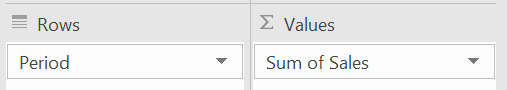
Previously, this Pivot Table yields all the data we would have been able to extract from the budget file. If we wanted to add, Year, Month, and Month Name we would need to add 3 new columns to the budget file (and repeat each time we received a new file from the budget team).

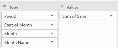
Let's look at how the world has changed. In the Pivot Table Fields List, add Start of Month, Month and Month Name to rows.

If you do nothing else in Power Pivot, when your Lookup Table has unique values, load your files and build the relationships to remove VLOOKUPs. You will find immediate improvement in the performance of your files.
The Power Pivot Data Model compresses data 7 to 10 times smaller than the same data in native Excel. Native Excel uses the in-memory analytics engine to store data in memory (hence why large files with complex formulas or multiple Pivots receive resource error messages).
In this lesson, you learned how to:
- Navigate in Power Pivot;
- Build relationships using Power Pivot;
- Interpret the Connector in Power Pivot;
- Create 1 Pivot Table using 2 data sets; and,
- The value of performing calculations, such as VLOOKUP, in Power Pivot instead of native Excel.
SOLUTION
Prior post: Power Pivot Date Table
Next post: 2 Data Tables on 1 Pivot Table
💬 Questions or challenges can always be addressed in the comment section below.
No comments:
Post a Comment