Transforming a PDF

For this next exercise, we will build our PowerBI skills further, automating cleaning up the data within the PowerBI application. The post is a continuation of the work that was started in the post, Convert PDF Using PowerBI. In the original exercise, we took a PDF file and converted it to a visualization using PowerBI; now, we will perform transformation work to the PDF file before reloading it to the data visualization. 

The Scenario

In this series of exercises, the goal is to pull a list of all names from a PDF. In the first exercise, we just loaded the data as is; however, if you compare the source PDF file to the final visualization, many of the names are missing, with the PowerBI visualization matrix only displaying the names that start from the PDF section Randy Travis.

To begin the transformation process, let's start where we left off in the prior PDF lesson: with the Solution file. Open the Solution PowerBI file (or your prior exercise workbook), and then navigate to the PowerQuery Editor within PowerBI by selecting the query Table025 (Page 11). Right click and select "Edit Query".

---

Process the data

You've now entered the Power Query Editor: the same one used for Power Query in Excel. 

Looking at the data, there's a few things we need to address to get to our goal: a list of all names.

• Column2 has a rouge name (Nicole Lopez).
• Column1 includes characters (i.e, 2019-10) preceding the name.
• Columns 1, 2 & 6 each contain names, but we them all in a single list..

Let's tackle these clean-up items one-by-one. 

Addressing the rouge Name in Column2

To fix the name hanging out by itself in Column2, we will combine Column1 and Column2, by adding a Conditional Column. The Conditional Column will be called "1st column" and will look at Column2 and if Column2 has a value of null, then populate [1st column] with the value from Column1. If not null, then it will populate the value from Column2. This is very similar to the manual Excel process of creating a new column and then using an IF statement to populate each row. 

ln the PowerBI Power Query Editor ribbon, select Add Column, then Conditional Column,

When the "Add Conditional Column" menu opens, populate the fields as shown in the image below. Remember Power Query is case sensitive so "null" must be lowercase. 

After selecting "OK", there will be an extra column named [1st column]. By default, Power Query always adds new columns to the far right of your dataset. 

Now, we've got the names from Column1 and Column2 in one column. However, we also have extra data (i.e., 2019-10) in the column that we need to remove. Time for the second cleanup exercise.

Remove digits preceding names

To isolate the name, we need to remove the digits that precede them (i.e., 2019-10). We will use something similar to Excel's Text to Columns: Split Column by Delimiter. 

Click on the header for the new column, [1st column], highlighting the entire column. In the ribbon, on the Home menu, select the Split Column option, then By Delimiter.

In the Split Column by Delimiter menu, select Space from the drop down menu, and then Left-most delimiter. This will split [1st column] in to two columns based on the first space it finds, reading left to right. {I love the extra flexibility Split Column offers, such as Left-most, compared to the similar Excel version!}

In the new column [1st column.2], the first few rows look as expected and appear to have achieved the objective. However, as you scroll further down, you can see that "Nicole" is separated from her last name "Lopez". This happened because "Nicole Lopez" didn't have a space in front of it, and so the Left-most Space used to split the column was the space between "Nicole" and "Lopez". There are several approaches we could take to address this issue, but for this exercise we will focus on modifying an existing formula.

Modify Formula for Conditional Column

When we created [1st column], we used the Conditional Column menu to create an if statement that returned Column2's value when Column2 had a value. But, if instead of returning just Column2's value, we returned Column1 + Column2, then the data in Column2 will look the same as Column1. Since the columns look the same after the revision, the Split Column by Delimiter step will work the same, resulting in the correct result for the name of "Nicole Lopez".

If you haven't turned on your formula bar, go to the View menu on the ribbon and check the box "Formula bar". This is a one time set-up.

Now in the Applied Steps area of the Power Query Editor, select the step named "Added Conditional Column". 

Selecting an Applied Step changes the Preview to show the data how it looked after that step was performed, but before the subsequent steps. It also updates the formula bar to show the M language formula used to create that step. 

Good news is that you don't have to learn the M language in order to make some easy changes using it. In this case, we are going to modify the portion referring to the results of the new Conditional Column. In the formula above, it says if [Column2] is not null then [Column2]. We'll modify the very end of the formula to say "then [Column1]&[Column2]". You can make that change by directly typing in the formula bar above.

An ampersand is used in Power Query to indicate "and", or to join two words together. After pasting in the "[Column1]&" in the formula bar, it should read as follows. Now if we look at the [1st column], all columns have a "2019-##" and a name. 

In the [1st column] there is one last issue left to clean-up: there is a space missing on Row 11. Similar to above, we are going to manually type in the instructions to the formula bar. To add text to a column in Power Query, surround texts by quotation marks. Adding a space then is, " "; quotation marks with a space between them. The final modified formula looks like this, and the person listed on Row 11, aligns with the other rows. Even better, you've created the rules once, and if this ever occurs again in the future, the directions are written, and the process will be lightning fast.

Remove other columns

Power Query works faster when you remove any unnecessary columns. Since for this exercise all we need is a final list of names, we can tell Power Query to remove all other columns, leaving only the [1st column.2]. Do so by selecting [1st column.2], right clicking and selecting the option "Remove Other Columns". 

Combine columns within the same query

We now have a column that shows all the cleaned-up names from Column1, but we need to add to it the names in Column6. The good news is that the Column6 names are already cleaned up, so no work is required there, 

For this trick, I'm going to show you how to append a Table within the same query, combining the new [1st column] with Column6; in plain English, I'm going to show you how to get the new Column1 and Column6 in to a single name column.

Let's start by renaming [1st column.2] to "Column6". This aligns the name of the two columns that contain names: the column we cleaned up and the original column6. The append functions combines columns together based on their headers, so ensure it's spelled exactly the same way including capitalization. Rename a column by double clicking the header. 

Next, we will use the append function. In the ribbon, under Home, you'll find Append on the far right. Select the first option, Append Queries. Append makes a current list longer, by lining up data from multiple columns with the same headers.

In the pop-up Append menu, in the Table to append dropdown, select the current query, Table025 (Page 11). This option results in the query appending to itself. Notice in the preview area how the list of names restarts on row 17.

What we need to do next is to change the Append formula manually to look at a version of the query where the original Colunm6 is still included, and then Append that version of the Table to the version that has Column1 renamed as Column6. Essentially, next we need to combine both lists of names from the original columns 1 and 6. Instead of writing the formula from scratch, we used the Power Query menu options to do the hard work, and we will tweak the formula for this scenario. I totally geek out on tricks like these, and how much they expand your capabilities in Power Query, with minimal investment. 

If you select on the Applied Step for Appended Query, it will show the formula for that step in the formula bar. Reading the formula from left to right it says "Combine Tables that are located at the Applied Step Renamed Columns with the Table at the same Applied Step Renamed Columns". 

To modify the formula, we will replace one of the Renamed Columns references with a reference to an Applied Step that contained Column6. We got rid of Column6 when we performed the step Removed Other Columns; so a Step where Column6 was still in the Table was the Changed Type1 Step. 

So while in the Appended Query Applied Step, we are going to replace one of the references to Renamed Columns with the Changed Type1 step. Remember that Power Query is case sensitive, so be sure to spell exactly as shown. The # proceeding the reference indicates that you are referring to a Step in the query, and if a Step is more than one word, quotation marks should surround it. Here's how the final modified formula will look.

Alternatively, you also could have swapped the order and placed Changed Type1 first and Renamed Columns last.

Now that you've manually updated the formula, you'll notice two changes: 1) it's pulled back in all the rows that you removed previously, and 2) Column6 now includes names from both columns of the original table. 

Repeat the step to Remove Other Columns, keeping only Column6, and you have a single clean list of names, converted from a PDF to a Power BI query.

Prior post: Convert PDF using PowerBI

Next post: Coming soon

A table is not a Table

In this post, we will dig deeper, to discover why an Excel Table is much more powerful than just formatting.

---

What is a table?

Let's start with some basic definitions.

 

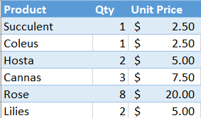
In Excel, you can freely structure content within cells; cell A3 below is just data. 

 

When you highlight cells A3:C5, the data becomes part of a range. 

The range becomes a table when every column has a header (note the lower case "t"), such as A3:C5.

In a table structure, a user might understand that row 3 contains headers, but Excel doesn't know that. Excel also doesn't understand that cell B4 is a Qty of Succulents.

---

Converting a table to a Table

A table can easily be converted to an Excel Table by selecting the table range and then pressing Ctrl + T. It can also be created from the Home menu by selecting "Format as Table", or from the Insert menu by selecting Table, then Table. The fact that Excel gave us 3 ways to create a Table signals its power.

Once the Table is created, you'll notice cosmetically that the data has been formatted. My default layout changes the rows to blue and white, alternating between each row (i.e, banded rows).

Most importantly, when you select anywhere in the Table, a new Table Design menu becomes available on the ribbon. This is an easy way to confirm that all your data has been picked up in the Table. By using End + arrow keys, you can quickly scroll around the edges of the Table and ensure all data which should be included has been.

---

What is a Table?

Now that you've created a Table, let's explore some of the key features of a Table.

Structure

An Excel Table is structured. The first row is always the Header row. Everything beneath a header relates to that header; for example, beneath the Product header are types of products. 

No cell references

Since Excel understands a Table's structure, you can reference Header names directly when writing formulas. For example, you could write a formula for Total Sales as  =[@Qty]*[@[Unit Price]]. 

In Table formulas, the @ symbol indicates that the formula should be applied @ the current row; it precedes the column name. Column names are in brackets []; if there is a space in the column, two sets of brackets are used, such as in [@[Unit Price]].

This is a significant deviation from the traditional formulas of =B4*C4, but results in much more intuitive formulas which explain what's happening (Qty * Price). When the data is located separate from the formula such as on another worksheet, the efficiency created by using Excel Tables is even more evident.

Formula auto-calculation

When a formula is entered in to a Table, the formula is automatically copied down to the remainder of the Table rows and gets Power-calculated. To me, this is personally the best benefit of using Tables.  I work with lots of large data sets containing lookups, SUMIFs, and nested IFs. Copying down a new formula can take a few minutes, or cause Excel to stop responding; but, when using the exact same data formatted as an Excel Table, I rarely ever have issues and formulas take a couple of seconds, no matter how complex. 

New rows

When adding a new row to a Table, any formulas automatically copy down. Give it a try by downloading the exercise file below, then copy the additional data and paste in cell A10.

                                                                   ↑

Headers

Since Excel knows the Headers, there's no need to Freeze Panes. When you scroll down in the Table, the Headers float to the top replacing the traditional A:Z column headers.

Ranges defined

Since Excel knows how a Table is structured, as long as your cursor is anywhere inside Table, a few things are easier than ever:

- Sorting: Just select Sort; no need to highlight a range.

- Pivot Tables: Range is automatically the entire range of the Table.

- Power Query: When loading from the current workbook, Power Query needs the data as a Table.

---

In this lesson, you learned:

• The difference between a table and an Excel Table;
• How to create a Table; and
• The functions of Table including a structure Excel can read, no cell references, formula auto-creation, auto add formulas for new rows, scrolling headers, and a defined named range.

SOLUTION

 

Prior post: Error Checking

Next post: Query Dependencies

What's killing My Excel?

Across the globe, Excel crashing is an accountant or analyst's bane. I've been there and know how exhausting it can be.  Fortunately (knock on wood), I've found some tips which have virtually eliminated crashing for me.  

• Get 64-bit Excel

• Disable add-ins

• Prioritize Excel

• Check your resource monitor

---

Get 64-bit Excel

The #1 way to fix Excel crashing issues is to install the 64-bit version of Excel on Office 365.  

By default, IT departments across the globe install the 32-bit version of Excel on Office 365.  While that works for most, Excel's 32-bit version is not sufficient for running the more complex Excel workbooks used by finance and accounting teams.  See this Microsoft Office article about why multiple Pivot Tables, slicers and VLOOKUPs can constrain your Excel resources.   

Finance and Accounting users are frequently the largest Excel consumers, but your IT support team may not realize it when deploying PCs to users.  If your Finance and Accounting teams aren't using 64-bit Excel today, there may be some support team resistance to making the change and deploying 64-bit.  Historically, Microsoft Office recommended 32-bit installs by default; however, it did not apply to power users like Finance and Accounting teams.  Here's a link to another Microsoft Office article which might help persuade.

Incapability with existing add-ins, such as Hyperion Essbase, is the primary issue which may need to be addressed. 

• First, I recommend seeing if there is a 64-bit version of your add-in.
• If not, consider installing anyway and testing the impact.
• If impacted, explore with your IT team other solutions, such as a 32-bit Excel version with the add-in installed inside a Citrix environment and the 64-bit Excel version on your desktop.

If you are experiencing install setbacks, don't give up; I assure you the 64-bit version is worth it.  While you wait for IT to validate add-ins, try one of the other solutions below. 

---

Disable Add-Ins

Excel Add-ins sometimes behave badly, especially when the version of Excel the add-in was built on and the current user version of Excel deviate.  This seems to be especially true in the Office 365 environment where updates can occur monthly.

Initially, try disabling all add-ins and turning them on only when needed.  To effectuate, in Excel go to File, Options, Add-ins, Manage, Excel Add-ins, Go.  Uncheck all the add-ins.  Next, repeat these steps, but select Manage, COM Add-ins, Go.

---

💥BEST PRACTICE TIP
Speed up the add-in disabling process by adding a short-cut to your Excel Quick Access Toolbar.  In Excel, go to File, Options, Quick Access Toolbar, Choose commands from: All Commands, Add-ins (the first one, which has no icon & a drop down menu). 💥

---