The CPA Revolution

Query dependencies

Just joining the blog? Explore prior lessons here.

When you have multiple queries which depend on each other, it's important to understand those connections, especially if you weren't the person who originally wrote the set of queries.

Power Query's Query Dependencies creates a visual map to display how each query is connected to the others.

Query Dependencies

To view Query Dependencies, open the Power Query Editor, and on the View menu select "Query Dependencies" on the far right.

Below is an example of a set of queries. Notice first that the query "Calendar" is not connected to any other query. Then note how the Current Workbook serves as the central source for the remaining displayed queries. The query "Path2" is the foundation for the next queries. If you modified "Path2" it could impact all the queries downstream culminating in to the "Newest Transactions" query which is built from combining all the connected files upstream of it ending in the final query "Working_Budget_Query".

In this lesson, you learned how to:

How to view Query Dependencies; and
How to interpret the query dependency map.

Prior post: A table is not a Table

Next post: Combine all files in a folder, Coming October 25

A table is not a Table

In this post, we will dig deeper, to discover why an Excel Table is much more powerful than just formatting.

What is a table?

Let's start with some basic definitions.

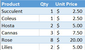
In Excel, you can freely structure content within cells; cell A3 below is just data.

When you highlight cells A3:C5, the data becomes part of a range.

The range becomes a table when every column has a header (note the lower case "t"), such as A3:C5.

In a table structure, a user might understand that row 3 contains headers, but Excel doesn't know that. Excel also doesn't understand that cell B4 is a Qty of Succulents.

Converting a table to a Table

A table can easily be converted to an Excel Table by selecting the table range and then pressing Ctrl + T. It can also be created from the Home menu by selecting "Format as Table", or from the Insert menu by selecting Table, then Table. The fact that Excel gave us 3 ways to create a Table signals its power.

Once the Table is created, you'll notice cosmetically that the data has been formatted. My default layout changes the rows to blue and white, alternating between each row (i.e, banded rows).

Most importantly, when you select anywhere in the Table, a new Table Design menu becomes available on the ribbon. This is an easy way to confirm that all your data has been picked up in the Table. By using End + arrow keys, you can quickly scroll around the edges of the Table and ensure all data which should be included has been.

What is a Table?

Now that you've created a Table, let's explore some of the key features of a Table.

Structure

An Excel Table is structured. The first row is always the Header row. Everything beneath a header relates to that header; for example, beneath the Product header are types of products.

No cell references

Since Excel understands a Table's structure, you can reference Header names directly when writing formulas. For example, you could write a formula for Total Sales as =[@Qty]*[@[Unit Price]].

In Table formulas, the @ symbol indicates that the formula should be applied @ the current row; it precedes the column name. Column names are in brackets []; if there is a space in the column, two sets of brackets are used, such as in [@[Unit Price]].

This is a significant deviation from the traditional formulas of =B4*C4, but results in much more intuitive formulas which explain what's happening (Qty * Price). When the data is located separate from the formula such as on another worksheet, the efficiency created by using Excel Tables is even more evident.

Formula auto-calculation

When a formula is entered in to a Table, the formula is automatically copied down to the remainder of the Table rows and gets Power-calculated. To me, this is personally the best benefit of using Tables. I work with lots of large data sets containing lookups, SUMIFs, and nested IFs. Copying down a new formula can take a few minutes, or cause Excel to stop responding; but, when using the exact same data formatted as an Excel Table, I rarely ever have issues and formulas take a couple of seconds, no matter how complex.

New rows

When adding a new row to a Table, any formulas automatically copy down. Give it a try by downloading the exercise file below, then copy the additional data and paste in cell A10.

↑

Headers

Since Excel knows the Headers, there's no need to Freeze Panes. When you scroll down in the Table, the Headers float to the top replacing the traditional A:Z column headers.

Ranges defined

Since Excel knows how a Table is structured, as long as your cursor is anywhere inside Table, a few things are easier than ever:

- Sorting: Just select Sort; no need to highlight a range.

- Pivot Tables: Range is automatically the entire range of the Table.

- Power Query: When loading from the current workbook, Power Query needs the data as a Table.

In this lesson, you learned:

The difference between a table and an Excel Table;
How to create a Table; and
The functions of Table including a structure Excel can read, no cell references, formula auto-creation, auto add formulas for new rows, scrolling headers, and a defined named range.

SOLUTION

Prior post: Error Checking

Next post: Query Dependencies

Error checking

Just joining? Explore prior lessons here.

If you've played around with Power Query a bit, you may have experienced query errors, where loading a query shows a message such as "4 errors". This post shows an easy way to proactively check for errors before loading.

The Data

For this exercise, we will use a simple data set of Actual Sales which contains two columns: Date & Sales. Download the file below, or follow along with a similar workbook of your own.

↑

The Problem

If you look at the dataset, the yellow highlight is a date error, since Excel isn't ready yet for year 20122.

When the data is loaded in to a Pivot Table, the Pivot isn't going to treat it as a date as shown below.

Similarly when the same data is loaded in to Power Query, and the column is tagged as Data Type "Date", then Power Query is going to treat it as an error. If you don't catch it at the onset, when the query is loaded, you'll note an error message similar to below.

The Solution

Identifying the errors proactively, before loading a query, is ideal. To do so, we need to modify the View. Inside the Power Query Editor, on the View tab, there are two options which will provide the error information we seek: "Column quality" and "Column profile".

Column Quality provides three quick facts at the top of each column: they are the percent of data which is Valid, an Error, and Empty. By focusing on the Error metric, it is easy to identify that this query has errors in columns "Date of Sale" and "Start of Month".

Then you can focus on those columns and identify where in the column the error is occurring. This leads to one of the following decisions which will need to be made:

Accept the error, knowing the data won't present appropriately in a Pivot, the Data Model, or a Measure.
Remove the errors using Power Query by right clicking on the column header and selecting "Remove Errors", but this impacts data quality and completeness.
Fix the error at the source. Now that you know where the error is, it will be easier to go back to the source and fix the problem. When you are dealing with very large data sets, finding the problem is half the battle.
Fix the error using Power Query. Using transformation tools, such as Replace Values, the error can be corrected before the Changed Type step.

Column Profile

In addition to the Column Quality option, another View which was enabled above was the Column Profile. Where Column Quality stays on for each column, Column Profile only displays information when an individual column header is selected.

When selecting the Date of Sale column, on the left side are statistics about the selected column including row count and number of errors. However, since there is an error in this column, Column Profile doesn't provide any additional information.

Let's contrast this with the Column Profile of a column without errors, such as the Sales column.

When a column has no errors, the Column Profile view is able to provide more information as shown above. The left side has more statistical data such as the number of empty rows, number of distinct or unique values, or the average of all values. On the right side, there's a distribution graph showing the frequency of each value.

One of these two views is sure to be helpful in your Power Query journey.

In this lesson, you learned how to:

Find errors using Column Quality and Column Profile; and,
Address errors using four alternative approaches.

SOLUTION

Prior post: Relationship Problems

Next post: A table is not a Table

Relationship problems

Just joining the blog? Explore prior lessons on Relationships here.

Ah, relationships: they always seem to have at least some problems.

In Power Pivot, the most obvious alert to a relationship problem is when all the values in a Pivot Table are the same.

Let's walk through a few examples illustrating how things go wrong, so you can spot and solve issues when they occur in your own data sets.

The Data

For this exercise, there are two data sets: a Costs Table and a Sign Table. Download the data file by selecting the icon above the arrow below.

↑

Let's explore the data in the Tables. The Sign Table is a Lookup Table for the natural sign based on transaction type. There are the two typical accounting transaction types (debit and credit) plus an additional type, Other (for statistical transactions).

The Costs Table contains 12 accounting transactions; most transactions have a typical Transaction Type of Credit or Debit, but 2 are listed as Total and 1 is listed as Zero.

In native Excel, if you did a VLOOKUP to find the sign for the last transaction with a Transaction Type of Zero, the result would be #N/A.

How will a Power Pivot Table handle the same exercise?

How should the Pivots be set-up to obtain the correct count of transactions by type?

Lookup Table field as value

On the Pivots tab, 2 Pivot Tables have been built which essentially are trying to gather the same information: what is the count of the type of each transaction? The first set is pulling in to the rows area Transactions Type from the Costs Table (Data Table). The second set is pulling in Type from the Sign Table (Lookup Table).

Let's look first at the impact of pulling in to the values area of each Pivot Table the type from the Lookup Table (Type from the Costs Table).

Immediately noticeable is the left Pivot showing the count of Type as 3 in each row. Since Zero occurs only once in the Costs data, how can there be a count of 3? If the Grand Total is 3, how can each row also be 3?

Power Pivot gives us a hint to why the left Pivot is returning 3 for each Transaction Type. When the Relationships alert shows up, it usually means we need to look at our relationship or in this case, build one.

Build the Relationship

The relationship error message isn't extremely helpful; selecting Auto-Detect shows "No new relationships found". Selecting Create opens a box to Create Relationship, but requires understanding which type should be the Foreign and Primary keys. I prefer instead to use the Power Pivot menu.

Let's build the relationship by going to the Power Pivot menu on the ribbon, then select Manage. Inside Power Pivot, select the Diagram View. Remember that the Data Table is the Costs Table and the Lookup Table is the Sign Table. So we'll need to have the Costs Table lookup to the Sign Table. To do so, in the Costs Table, select Transaction Type and drag over to the Sign Table Type field. This connects the two fields establishing a Relationship.

Looking at the Pivot Tables now, you'll note nothing has changed. Further exploration is required.

Data Table field as value

In the exercise above, type was pulled in to the Pivots from the Lookup Table, Sign. This returned a value of three which represents the number of types listed in the Lookup Table (Credit, Debit, Other). Each type being represented once, the Pivot on the right provided the correct count of the lookup, but not the count of the transactions by type.

Now let's pull in to each Pivot the Transaction Type from the Costs query.

Both Tables show a Count of 12. The left Pivot shows the count for Zero and Total, whereas the right Pivot only shows Blank, since those labels aren't in the Sign Table. On the surface, it seems like the left Pivot is the correct approach.

Let's perform one more test.

The Final Test

Let's add the Sign to both Pivots.

Now this view highlights an important issue with the left Pivot. While it's not returning a result of 3 in each row of the Pivot, showing 1 as the result is also incorrect. If you were to write Measures off the Table like this, your results would be inaccurate.

Why did this return the wrong result? The cause is because the left Pivot is asking for data from the Lookup Table (Sign) and from the transaction table (Transaction Type). In Power Pivot, Lookup Tables can see in to Data Tables, but Data Tables can't see in to Lookup Tables. Regardless of the rows field, the relationship flows down from the Sign Table to the Costs Table.

When I first started using Power Pivot, I frequently had results where all rows were the incorrectly the same frustrating number.

💥BEST PRACTICE TIP

Always use the columns from the Lookup Table, not the Data Table, as the fields in the Pivot. If the columns from the Data Table are used, the Pivot can not correctly see the Lookup Tables or other Data Tables, and the Pivot Table will return inaccurate results.💥

Now that you know the Best Practice Tip, the right approach to building these Pivots was the Pivot on the right. Since the values area includes fields from both the Lookup and Data Tables, the rows (and column) areas can only include fields from the Lookup Table.

In this lesson, you learned:

Always use the columns from the Lookup Table, not the Data Table, as the fields in the Pivot;
Always build relationships where the data table lookups to the lookup table; and
Just because it looks right, doesn't mean it is. Robustly test for accuracy.

SOLUTION

Prior post: Measures: Right& Wrong

Next post: Error checking

Measures: Right & Wrong

Explore prior lessons on Measures here.

Measures are very powerful custom functions used inside Pivot Tables. However, when I started using them, I found myself getting easily twisted up between when to use SUM vs SUMX.

I built a cheat sheet to help me remember. Hope it helps you too.

The Cheat Sheet

Table1 below has Qty & Price. To calculate Sales, you could add a column to multiple Qty * Price as shown. However, calculating a value for each row uses a lot of memory, especially when you have lots of data.

Measures are a much more efficient way to calculate values for large data sets. There are several ways to write Measures to calculate sales, but only one way which avoids adding the Sales column to the Table above and results in the correct Grand Total of 20.

Note first, in all cases the sales for Item A have been calculated correctly, as well as Item B. The difference is the Grand Total. Adding 11 to 9 is 20, so with this small dataset this is an easy approach to check if a Measure is returning the correct result.

Sum of Sales

Sum of Sales was calculated the traditional way, by pulling the Sales column in to the Values section of the Pivot Table. It achieves the correct result. However, it can't be inserted inside another function such as Item Sales as a % of Total Sales. It also requires having a Sales column in the Table which isn't efficient.

Sales SUM

The next approach does not need a Sales column in the Table. This is a Measure which multiplies Price times Qty. This yields the correct result for the Sales of Items A and B, but the Grand total takes the combined price of Items A & B (11+3=14) times the combined Qty (1+3=4), which equals 14*4=56. This is incorrect as the sum of the sales for A (11) & B (9) is 20.

Sales Sum of Sum

When writing a Measure for the first time, I like starting with something I know will work and then building out from there. The Sales Sum of Sum utilizes the Sales column that was added to Table1. Taking the Sum of the Sales column yields the correct Grand Total. However, having an extra column isn't ideal.

Sales SUMX

SUMX is an iterator: it goes through each row and sums it. First the Sum of the Sales column was calculated, which was 20, then SUMX went through each row of the query and summed the sales. Effectively, this doubled each Item's sales. Using the Sales column in Table1, SUMX summed the total sales in row A & B, essentially doubling total sales. Wrong answer but an iterator has potential.

SUMX Sales

Now that's the right answer! But, it's using the Sales column again. However, it does tell us that SUMX could be used to get to the correct subtotal.

SUMX PQ

Finally, the sweet spot. SUMX PQ has the correct Grandtotal and does not require a Sales column added to the Table. This is the correct way to write a SUMX Measure.

Wrap-up

This cheat sheet shows all the wrong ways to write a Measure. When I tried to write DAX on the fly in the beginning, I've made every one of these errors. Happy DAX-ing!

In this lesson, you learned how to:

Write SUMX Measures the wrong way, and
Write SUMX Measures the right way.

SOLUTION

Prior post: M-language

Next post: Relationship problems

M-language

Just joining the blog? Explore prior lessons here.

When using Power Query, steps are written using the M-language. Learning a little bit about the M-language can really help expand your Power Query automation skills.

The good news is that most M-language questions can be solved by knowing 3 things.

1. M formulas can be found on Microsoft's website.

2. Steps can be performed first using the tools on the ribbon, and then adding M-language to tweak the final result (see example below).

3. The M-language is case sensitive.

Illustrative example

In this example, the user has a Variance and a Threshold and is trying to determine when a row is above the threshold.

In the Power Query Editor, first create a Conditional Column.

Create a step using the Add Conditional Column prompt. Enter the parameters as shown below to create a column "$ above threshold" which will look at the Variance YOY column. If the value is less than or equal to the value in the Threshold $ column, then the column will have a value of "No" for that row; if not, then the value will be "Yes".

After the column is created, you can look at the M-language in the formula bar. If the bar is hidden, on the ribbon, go to the View menu and check the box for Formula Bar as shown below.

The formula for the conditional column is provided below. The formula can be read as "in the table, add a column, after the Changed Type step. Name the column "$ above threshold". For each row, if the value in the Variance YOY column is less than or equal to the value in the Threshold $, then the value in the new column should be No, else it should be Yes".

Adding to the M-language

What the end user really wants is a column which looks at the absolute value of the Variance YOY and then evaluates if it's above the dollar threshold.

Using the Add Conditional Column prompt, there is no way to add an absolute value evaluation to the formula. However, it can be done in two steps:

Search on Microsoft's website for the M-language for absolute value;
Add the M-language for absolute value to the formula generated using the "Added Conditional Column" prompt.

Search for M-language

On Microsoft's website, in the "filter by title" box starting to type "Absolute" yields a Power Query M function, Number.Abs.

Reading through the description, it is clear Number.Abs is the function we are looking for to modify our existing M-language to calculate the absolute value of the Variance YOY column.

Adding M-language

Now returning to the Power Query Editor, and selecting the step "Added Conditional Column", the formula bar will once again show the function. Modify the formula by typing in Number.Abs (case sensitive) before the column reference for [Variance YOY]. Also surround [Variance YOY] in parens.

M-language with modification

M-language before modification

In this lesson, you learned how to:

Modify an existing M-language formula;
Locate new M formulas to enhance capabilities; and,
Check the case, since the M-language formula is case sensitive.

SOLUTION

Prior post: Calculated columns vs Measures

Next post: Measures: Right & Wrong

Calculated columns vs Measures

Just joining the blog? Explore prior lessons here.

When playing with the Power tools, there is often more than one way to tackle a task. Read further to explore the pros and cons of calculated columns and Measures.

For this exercise, we'll use the dataset below to find Total Sales for each product using calculated columns and then a Measure.

⇧

Calculated Column

A calculated column expands a dataset by adding an additional column. It's similar to native Excel where you would write a formula in a new column.

New users will feel more comfortable using calculated columns instead of Measures. However, there are some downsides to this approach which we'll explore further down. For now though, let's practice our Power Query skills by adding a calculated column.

Select the Download icon above the arrow ⇧ on the dataset above. With your cursor in the Table, load to Power Query by going to the Data tab and selecting From Table/Range.

Inside the Power Query Editor, on the Add Column tab, select Custom Column.

Create a "Total sales" column like the example below.

After selecting OK, the new Calculated Column has been added to our query.

Change the type of "Total sales" to Decimal Number and then Close & Load To, Table, New worksheet, Add this data to the Data Model, Load.

Advantages of using Power Query instead of native Excel to build the Calculated Column include:

Removes the potential for a formula to get altered accidentally;
Shrinks the file size, since Power Query uses xVelocity to compress data; and,
Allows processing of massive amounts of data since Power Query is limited only by the capacity of your machine, not Excel's ~1 million rows limit: 20 million rows, no problem.

However, it could be even better. Let's try it in Power Pivot.

Build a Power Pivot Pivot Table

Before we write a Measure, let's add a Pivot Table to our workbook, so we can see the results.

Choose to "Use this workbook's Data Model". This creates a Pivot Table using the data loaded in to Power Query.

In the PivotTable Fields, there may be 3 Sales_data sets to choose from when selecting fields for the Pivot.

Hovering over the name yields more information to distinguish between the data sources.

The first is the original Data Table which was loaded to Power Query.
The second is the query that was created in Power Query.
The third is the output of the query.

On the PivotTable Field List, select from the query "Sales_data 1" and pull Product in to the Rows area and "Total sales" in to the Values area.

Measure

Now, let's calculate Total Sales again, but this time using a Measure instead of a calculated column. The results will be the same, but Measures have additional advantages over native Excel and calculated columns.

The Measure will need to multiply Qty and Unit Price for each row of the data and then sum those products to get a grand total. To achieve this result, we will use a SUMX formula, which is an iterator formula, which iterates through each row of the Table and then sums the total.

The SUMX format is

= SUMX(Source Query, function to perform on each row before summing)

In our case, this roughly translates to

=SUMX(Sales_data 1, Qty*Unit Price)

Let's write the Measure.

On the Power Pivot menu, select Measures, New Measure.

Name the Measure, "Total sales Measure".
Start the formula with an equal sign.
SUMX first needs a table to reference, so type an open parenthesis, then 'Sales_data 1' followed by a comma.
Then, start the expression by typing Qty. Select 'Sales_data 1'[Qty], which is the quantity column from the query.
Add a multiplication sign.
Type "price" and then select 'Sales_data 1'[Unit Price].
Close parenthesis.

Check the formula and assign the value a category. Here's the solution.

=SUMX('Sales_data 1','Sales_data 1'[Qty]*'Sales_data 1'[Unit Price])

Return to your Pivot Table, and add in the new Measure.

Advantages of using Power Pivot Measures instead of native Excel or Power Query to build the Total Sales calculation include:

All the advantages listed above for calculated columns versus native Excel plus the following.
Measures use less memory than calculated columns.
The Power Pivot Data Model compresses data 7 to 10 times smaller than the same data in native Excel.

Native Excel uses the in-memory analytics engine to store data in memory (hence why large files with complex formulas or multiple Pivots receive resource error messages).

Measures can be reused in multiple Pivot Tables in the same workbook.
Measures can be referred to in other Measures. For example, if we had to add sales tax of 10%, a Measure could be written to take =Total Sales Measure * 10%.

MeasureNow, let's calculate Total Sales again, but this time using a Measure instead of a calculated column. The results will be the same, but Measures have additional advantages over native Excel and calculated columns.

The SUMX format is

= SUMX(Source Query, function to perform on each row before summing)

In our case, this roughly translates to

=SUMX(Sales_data 1, Qty*Unit Price)

Let's write the Measure.

On the Power Pivot menu, select Measures, New Measure.

Name the Measure, "Total sales Measure".
Start the formula with an equal sign.
SUMX first needs a table to reference, so type an open parenthesis, then 'Sales_data 1' followed by a comma.
Then, start the expression by typing Qty. Select 'Sales_data 1'[Qty], which is the quantity column from the query.
Add a multiplication sign.
Type "price" and then select 'Sales_data 1'[Unit Price].
Close parenthesis.

Check the formula and assign the value a category. Here's the solution.

=SUMX('Sales_data 1','Sales_data 1'[Qty]*'Sales_data 1'[Unit Price])

Return to your Pivot Table, and add in the new Measure.

Advantages of using Power Pivot Measures instead of native Excel or Power Query to build the Total Sales calculation include:

All the advantages listed above for calculated columns versus native Excel plus the following.
Measures use less memory than calculated columns.
The Power Pivot Data Model compresses data 7 to 10 times smaller than the same data in native Excel.

Native Excel uses the in-memory analytics engine to store data in memory (hence why large files with complex formulas or multiple Pivots receive resource error messages).

Measures can be reused in multiple Pivot Tables in the same workbook.
Measures can be referred to in other Measures. For example, if we had to add sales tax of 10%, a Measure could be written to take =Total Sales Measure * 10%.

In this lesson, you learned:

Calculated columns and Measures can return the same results;
The difference between creating a calculated column and a Measure;
The advantages of creating a Power Query calculated column instead of using native Excel; and,
The advantages of creating Measures instead of using native Excel or Power Query.

SOLUTION

Prior post: The Power of the Unpivot
Next post: M-language