The Power of the Unpivot

Just joining? Explore prior lessons here.

A colleague's jaw literally dropped when I showed him Power Query's Unpivot functionality.  Unpivot transformed many days of work in to a data analysis delivered within hours.

---

The Predicament

Visualize a report similar to the one below, containing 12 months of data.

The initial report provides data in an orderly and logical format, but it's very difficult to take this data and answer analytical questions such as:

• What's been the trend in Net sales, current year versus prior year?
• How have returns trended as a % of sales?
• What does the growth in sales look like in store versus online? 
• What would next year's monthly sales be if sales online grew 5%?

---

The Transformation

Transform the flat report to a Pivot Table.

The transformation step-by-step follows.

---

Load the initial report

Download the initial report by selecting the ↑ below.

                                                    ↑

To load the initial report to Power Query, start with your cursor inside the Excel Table, Initial_Table.  On the Excel ribbon, go to the Data tab and select "From Table/Range".

---

Process the data

Process the data using Power Query.

Modify the defaults
By default, PQ names the Query the Table name and assigns a Type to each column.

Rename the Query, "Report_data" by selecting the default Name and typing over with the new name.

 Delete the Applied Step "Changed Type" by selecting the Red X next to the "Changed Type" step.



Create a Month column
Select Column1 and then on the Transform tab, select Transpose.  This flips the Month+Year into the first column of the query.



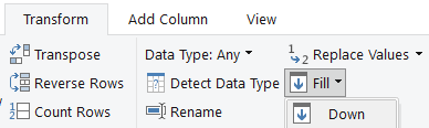
Select Column1 again and then on the Transform tab, select Fill, Down.




Some quick clean-up

On the Transform or Home tab, select "Use First Row as Headers".  When the headers are promoted, PQ applies the Change Type step.

Delete the Applied Step "Changed Type1" by selecting the Red X next to the "Changed Type1" step.

---

The Unpivot

Compare the query immediately before and after performing the Unpivot function.

Before

After

Unpivot took the column headers (with the exception of Column1 and Column2) and flipped them in to a new Attribute column, placing the amounts in to a single Value column.  Now, each row represents a single Value with a unique set of characteristics.  

To perform the Unpivot, select Column1 and Column2.  On the Transform tab, select "Unpivot Other Columns".

---

Polish the Presentation

Polish the query and enhance its analytical usefulness with these steps.

• Split the Month+Year in to separate columns.  Select Column1.  On the Transform tab, select Split Column, By Delimiter, Space & Left Most. 
• Rename the columns to Month, Year, Scenario, Sales type, and Amount.
• Change the data type of the Amount column to Decimal Number. 
• Filter out the Sales type of "Net sales".

Close & Load To a Pivot Table, or as a Connection Only, Add to the Data Model.

---

Analyze

Use a Pivot Table (and measures) to analyze the data.

---

In this lesson, you learned how to:

Change the layout of a query by unpivoting columns (flipping columns to rows);

Convert a flat table layout to a layout where each row represents a single value with a unique set of characteristics.  

Transform data using Fill Down and "Use First Row as Headers"; 

SOLUTION

Prior post: Distinguishing datasets in Power Pivot
Next post: Calculated Columns vs Measures